One Sample T-Test

Assumptions

As a parametric procedure (a procedure which estimates unknown parameters), the one sample t-test makes several assumptions. Although t-tests are quite robust, it is good practice to evaluate the degree of deviation from these assumptions in order to assess the quality of the results. The one sample t-test has four main assumptions:

• The dependent variable must be continuous (interval/ratio).
• The observations are independent of one another.
• The dependent variable should be approximately normally distributed.
• The dependent variable should not contain any outliers.

Level of Measurement

The one sample t-test requires the sample data to be numeric and continuous, as it is based on the normal distribution. Continuous data can take on any value within a range (income, height, weight, etc.). The opposite of continuous data is discrete data, which can only take on a few values (Low, Medium, High, etc.). Occasionally, discrete data can be used to approximate a continuous scale, such as with Likert-type scales.

Independence

Independence of observations is usually not testable, but can be reasonably assumed if the data collection process was random without replacement. In our example, we would want to select laptop computers at random, compared to using any systematic pattern. This ensures minimal risk of collecting a biased sample that would yield inaccurate results.

Normality

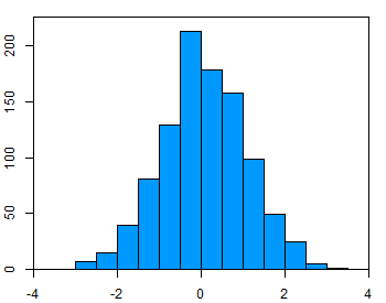
To test the assumption of normality, a variety of methods are available, but the simplest is to inspect the data visually using a histogram or a Q-Q scatterplot. Real-world data are almost never perfectly normal, so this assumption can be considered reasonably met if the shape looks approximately symmetric and bell-shaped. The data in the example figure below is approximately normally distributed.

Outliers

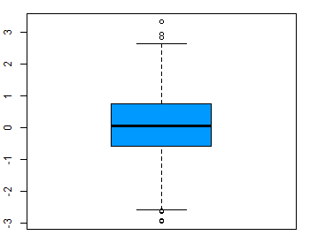
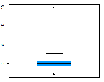
An outlier is a data value which is too extreme to belong in the distribution of interest. Let’s suppose in our example that the assembly machine ran out of a particular component, resulting in a laptop that was assembled at a much lower weight. This is a condition that is outside of our question of interest, and therefore we can remove that observation prior to conducting the analysis. However, just because a value is extreme does not make it an outlier. Let’s suppose that our laptop assembly machine occasionally produces laptops which weigh significantly more or less than five pounds, our target value. In this case, these extreme values are absolutely essential to the question we are asking and should not be removed. Box-plots are useful for visualizing the variability in a sample, as well as locating any outliers. The boxplot on the left shows a sample with no outliers. The boxplot on the right shows a sample with one outlier.

Procedure

The procedure for a one sample t-test can be summed up in four steps. The symbols to be used are defined below:

• \(Y\ =\ \)Random sample
• \(y_i\ =\ \)The \(i^{th}\) observation in \(Y\)
• \(n\ =\ \)The sample size
• \(m_0\ =\ \)The hypothesized value
• \(\overline{y}\ =\ \)The sample mean
• \(\hat{\sigma}\ =\ \)The sample standard deviation
• \(T\ =\)The critical value of a t-distribution with (\(n\ -\ 1\)) degrees of freedom
• \(t\ =\ \)The t-statistic (t-test statistic) for a one sample t-test
• \(p\ =\ \)The \(p\)-value (probability value) for the t-statistic.

The four steps are listed below:

• 1. Calculate the sample mean.
• \(\overline{y}\ =\ \frac{y_1\ +\ y_2\ +\ \cdots\ +\ y_n}{n}\)
• 2. Calculate the sample standard deviation.
• \(\hat{\sigma}\ =\ \sqrt{\frac{(y_1\ -\ \overline{y})^2\ +\ (y_2\ -\ \overline{y})^2\ +\ \cdots\ +\ (y_n\ -\ \overline{y})^2}{n\ -\ 1}}\)
• 3. Calculate the test statistic.
• \(t\ =\ \frac{\overline{y}\ -\ m_0}{\hat{\sigma}/\sqrt{n}}\)
• 4. Calculate the probability of observing the test statistic under the null hypothesis. This value is obtained by comparing t to a t-distribution with (\(n\ -\ 1\)) degrees of freedom. This can be done by looking up the value in a table, such as those found in many statistical textbooks, or with statistical software for more accurate results.
• \(p\ =\ 2\ \cdot\ Pr(T\ >\ |t|)\)    (two-tailed)
• \(p\ =\ Pr(T\ >\ t)\)    (upper-tailed)
• \(p\ =\ Pr(T\ <\ t)\)    (lower-tailed)

Once the assumptions have been verified and the calculations are complete, all that remains is to determine whether the results provide sufficient evidence to reject the null hypothesis in favor of the alternative hypothesis.

Interpretation

There are two types of significance to consider when interpreting the results of a one sample t-test, statistical significance and practical significance.

Statistical Significance

Statistical significance is determined by looking at the p-value. The p-value gives the probability of observing the test results under the null hypothesis. The lower the p-value, the lower the probability of obtaining a result like the one that was observed if the null hypothesis was true. Thus, a low p-value indicates decreased support for the null hypothesis. However, the possibility that the null hypothesis is true and that we simply obtained a very rare result can never be ruled out completely. The cutoff value for determining statistical significance is ultimately decided on by the researcher, but usually a value of .05 or less is chosen. This corresponds to a 5% (or less) chance of obtaining a result like the one that was observed if the null hypothesis was true.

Practical Significance

Practical significance depends on the subject matter. In general, a result is practically significant if the size of the effect is large (or small) enough to be relevant to the research questions being investigated.  It is not uncommon, especially with large sample sizes, to observe a result that is statistically significant but not practically significant.  Returning to the example of laptop weights, an average difference of .002 pounds might be statistically significant.  However, a difference this small is unlikely to be of any interest.  In most cases, both practical and statistical significance are required to draw meaningful conclusions.

Statistics Solutions can assist with your quantitative analysis by assisting you to develop your methodology and results chapters. The services that we offer include:

Data Analysis Plan

• Edit your research questions and null/alternative hypotheses
• Write your data analysis plan; specify specific statistics to address the research questions, the assumptions of the statistics, and justify why they are the appropriate statistics; provide references
• Justify your sample size/power analysis, provide references
• Explain your data analysis plan to you so you are comfortable and confident
• Two hours of additional support with your statistician

Quantitative Results Section (Descriptive Statistics, Bivariate and Multivariate Analyses, Structural Equation Modeling, Path analysis, HLM, Cluster Analysis)

• Clean and code dataset
• Conduct descriptive statistics (i.e., mean, standard deviation, frequency and percent, as appropriate)
• Conduct analyses to examine each of your research questions
• Write-up results
• Provide APA 7^th edition tables and figures
• Explain Chapter 4 findings
• Ongoing support for entire results chapter statistics

Please call 727-442-4290 to request a quote based on the specifics of your research, schedule using the calendar on this page, or email [email protected]