Conduct and Interpret a Canonical Correlation
What is Canonical Correlation analysis?
The Canonical Correlation is a multivariate analysis of correlation. Canonical analyzes latent variables, which researchers do not directly observe, but which represent multiple directly observed variables. The term also appears in canonical regression analysis and multivariate discriminant analysis.
Canonical Correlation analysis is the analysis of multiple-X multiple-Y correlation. The Canonical Correlation Coefficient measures the strength of association between two Canonical Variates.
A Canonical Variate is the weighted sum of the variables in the analysis. The canonical variate denotes as CV. Similarly to the discussions on why to use factor analysis instead of creating unweighted indices as independent variables in regression analysis, canonical correlation analysis is preferable in analyzing the strength of association between two constructs. This is such because it creates an internal structure, for example, a different importance of single item scores that make up the overall score (as found in satisfaction measurements and aptitude testing).
For multiple x and y the canonical correlation analysis constructs two variates CVX1 = a1x1 + a2x2 + a3x3 + … + anxn and CVY1 = b1y1 + b2y2 + b3y3 + … + bmym. The canonical weights a1…an and b1…bn maximize the correlation between the canonical variates CVX1 and CVY1. A pair of canonical variates forms a canonical root. This process repeats for the residuals, generating additional duplets of canonical variates until the cut-off value equals min(n, m). For example, when calculating the canonical correlation between three variables for test scores and five variables for aptitude testing, we extract three pairs of canonical variates or three canonical roots. Note that this is a major difference from factor analysis. In factor analysis, the method calculates the factors to maximize between-group variance while minimizing in-group variance. They are factors because they group the underlying variables.
Need help conducting your analysis? Leverage our 30+ years of experience and low-cost same-day service to complete your results today!
Schedule now using the calendar below.
Canonical variates are not factors. Only the first pair groups variables to maximize their correlation. The second pair uses residuals from the first pair to maximize their correlation. Therefore, canonical variates differ from factors in factor analysis. Additionally, the calculated canonical variates are automatically orthogonal, meaning they are independent of each other.
Like factor analysis, the central results of canonical correlation analysis are the canonical correlations, canonical factor loadings, and canonical weights. These can calculate d, a measure of redundancy. The redundancy measure is crucial in questionnaire design and scale development. It helps answer questions like, “Can I exclude one of the two scales to shorten my questionnaire when measuring satisfaction with the last purchase and after-sales support?”. Statistically, it represents the proportion of variance in one set of variables explained by the other set’s variance.
The canonical correlation coefficients test overall relationships between two sets of variables, while redundancy measures the strength of these relationships. Wilk’s lambda (U value) and Bartlett’s V serve as tests of significance for the canonical correlation coefficient. Wilk’s lambda tests the first canonical correlation coefficient, while Bartlett’s V tests all canonical correlation coefficients.
A final remark: Please note that the Discriminant Analysis is a special case of the canonical correlation analysis. You can replace every nominal variable with n different factor steps by n-1 dichotomous variables. The Discriminant Analysis is then nothing but a canonical correlation analysis of a set of binary variables. It is with a set of continuous-level (ratio or interval) variables.
Canonical Correlation Analysis in SPSS
We want to show the association between the five aptitude tests. We also want to show the association with the three tests on math, reading, and writing. Unfortunately, SPSS lacks a menu for canonical correlation analysis, so we need to run a couple of syntax commands. Don’t worry—it sounds more complicated than it is. First, open the syntax window by clicking File > New > Syntax.

In the SPSS syntax we need to use the command for MANOVA and the subcommand /discrim in a one factorial design. We need to include all independent variables in one single factor separating the two groups by the WITH command. The list of variables in the MANOVA command places the dependent variables first, followed by the independent variables. Avoid using the command BY instead of WITH, as it would separate the factors, similar to how they appear in a MANOVA analysis.
The subcommand /discrim produces a canonical correlation analysis for all covariates. Covariates are specified after the keyword WITH. ALPHA specifies the significance level required before a canonical variable is extracted, default is 0.25; it is typically set to 1.0 so that all discriminant functions are reported. Your syntax should look like this:

To execute the syntax, just highlight the code you just wrote and click on the big green Play button.

The Output of the Canonical Correlation Analysis
The syntax generates a large output, but we’ll focus on the important parts. It starts with a sample description and reports the model’s fit using Pillai’s, Helling’s, Wilk’s, and Roy’s multivariate criteria. While Wilk’s lambda is commonly used, all tests are significant with p<.05.
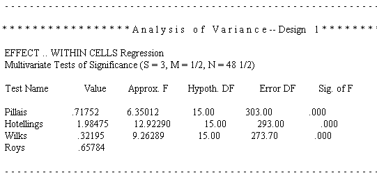
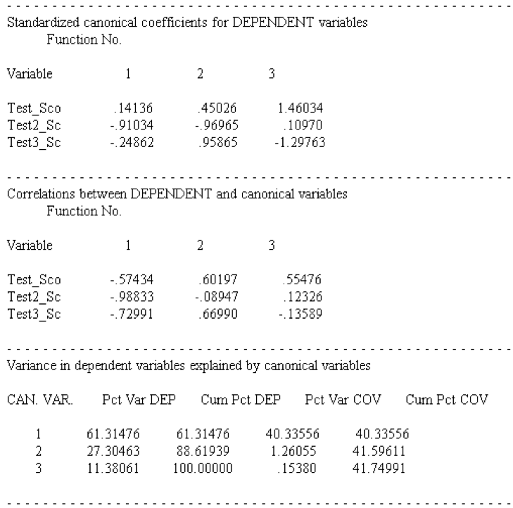
The next section reports the canonical correlation coefficients and the eigenvalues of the canonical roots. The first canonical correlation coefficient is .81108, with an explained variance of 96.87% and an eigenvalue of 1.92265. This confirms our hypothesis: the standardized test scores and the aptitude test scores correlate positively.
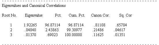
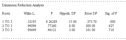
So far the output only showed overall model fit. The next part tests the significance of each of the roots. We find that of the three possible roots only the first root is significant with p < .05. Since our model contains the three test scores (math, reading, writing) and five aptitude tests, SPSS extracts three canonical roots or dimensions. The first test of significance tests all three canonical roots of significance (f = 9.26 p < .05), the second test excludes the first root and tests roots two to three, the last test tests root three by itself. In our example only the first root is significant p < .05.
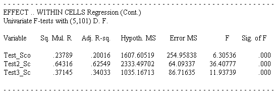
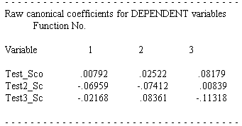
In the next parts of the output SPSS presents the results separately for each of the two sets of variables. Within each set, SPSS gives the raw canonical coefficients, standardized coefficients, correlations between observed variables, the canonical variant, and the percent of variance explained by the canonical variant. Below are the results for the 3 Test variables.
The raw canonical coefficients resemble the coefficients in linear regression and calculate the canonical scores.
The standardized coefficients (mean = 0, st.dev. = 1) are easier to interpret. Only the first root is relevant, as roots two and three are not significant. The strongest influence on the first root comes from the variable Test_Score (representing the math score).
The next section shows the same information (raw canonical coefficients, standardized coefficients, correlations between observed variables and the canonical variant, and the percent of variance explained by the canonical variant) for the aptitude test variables.

If you’re like others, you’ve invested a lot of time and money developing your dissertation or project research. Finish strong by learning how our dissertation specialists support your efforts to cross the finish line.