Conduct and Interpret a Linear Regression
What is Linear Regression?
Linear regression is the most basic and commonly used predictive analysis. Researchers use regression estimates to describe data and explain the relationship between one dependent variable and one or more independent variables. At the center of the regression analysis is the task of fitting a single line through a scatter plot. The simplest form with one dependent and one independent variable is defined by the formula y = a + b*x.
Key Concepts and Stages of Linear Regression Analysis
Sometimes, researchers refer to the dependent variable as the endogenous variable, prognostic variable, or regressand. The independent variables are also called exogenous variables, predictor variables or regressors.
Stages of Linear Regression Analysis
However Linear Regression Analysis consists of more than just fitting a linear line through a cloud of data points. It consists of 3 stages: 1) analyzing the correlation and directionality of the data, 2) estimating the model, i.e., fitting the line, and 3) evaluating the validity and usefulness of the model.
Major Uses of Regression Analysis
There are three major uses for Regression Analysis: 1) causal analysis, 2) forecasting an effect, 3) trend forecasting. Other than correlation analysis, which focuses on the strength of the relationship between two or more variables, regression analysis assumes a dependence or causal relationship between one or more independent and one dependent variable.
Firstly, it might be used to identify the strength of the effect that the independent variable(s) have on a dependent variable. Typical questions are what is the strength of relationship between dose and effect, sales and marketing spending, age and income.
Secondly, it can be used to forecast effects or impacts of changes. That is, regression analysis helps us to understand how much the dependent variable will change when we change one or more independent variables. Typical questions are, “How much additional Y do I get for one additional unit of X?”.
Thirdly, regression analysis predicts trends and future values. Researchers can use regression analysis to obtain point estimates. Typical questions are, “What will the price for gold be 6 month from now?” “What is the total effort for a task X?“
The linear Regression in SPSS
The research question for the Linear Regression Analysis is as follows:
In our sample of 107 students can we predict the standardized test score of reading when we know the standardized test score of writing?
Checking for a Linear Relationship in the Data
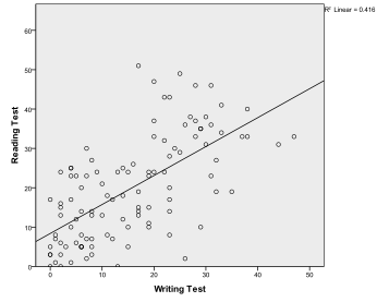
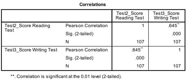
The first step is to check whether there is a linear relationship in the data. For that we check the scatter plot (Graphs/Chart Builder…). The scatter plot indicates a good linear relationship, which allows us to conduct a linear regression analysis. We can also check the Pearson’s Bivariate Correlation (Analyze/Correlate/Bivariate…) and find that both variables are strongly correlated (r = .645 with p < 0.001).
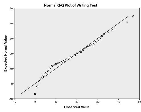
Secondly, we need to check for multivariate normality. We have a look at the Q-Q-Plots (Analyze/Descriptive statistics/Q-Q-Plots…) for both of our variables and see that they are not perfect, but it might be close enough.
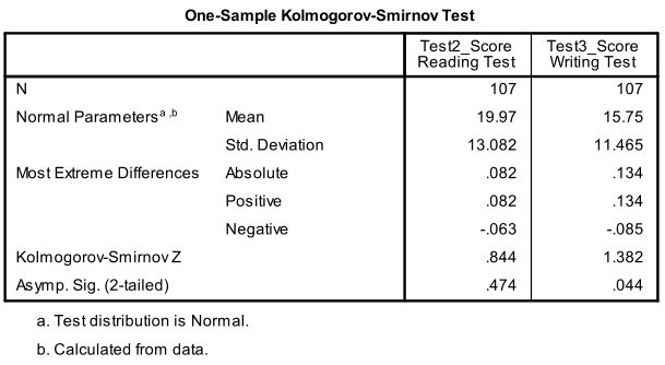
We can check our ‘eyeball’ test with the 1-Sample Kolmogorov-Smirnov test (Analyze/Non Paracontinuous-level Tests/Legacy Dialogs/1-Sample K-S…). The test has the null hypothesis that the variable approximates a normal distribution. The results confirm that the reading score follows a multivariate normal distribution (p = 0.474), while the writing test does not (p = 0.044). To fix this problem we could try to transform the writing test scores using a non-linear transformation (e.g., log). However, we do have a fairly large sample in which case the linear regression is quite robust against violations of normality. It may report too optimistic T-values and F-values.
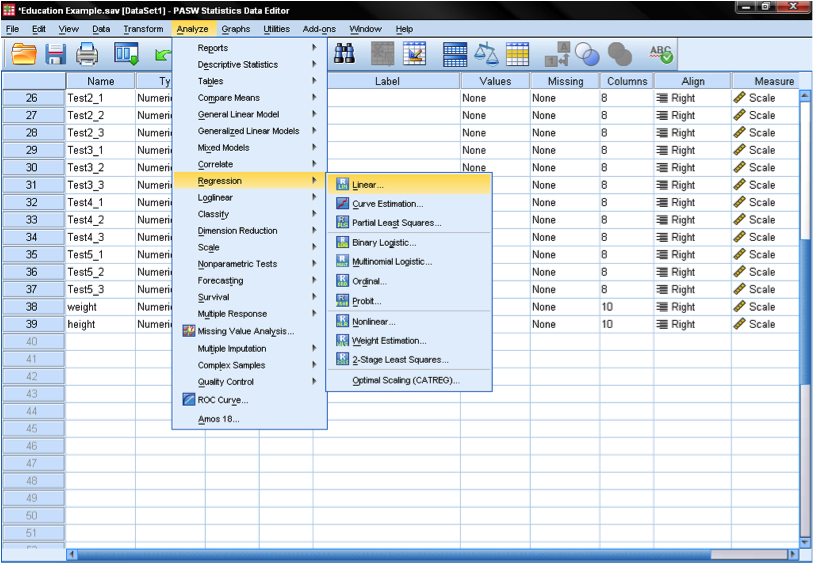
We now can conduct the linear regression analysis. You can find linear regression in SPSS under Analyze → Regression → Linear.
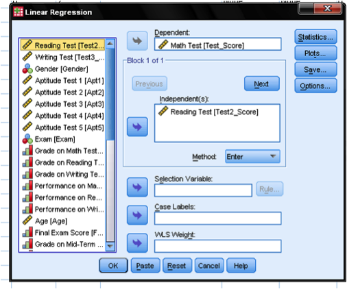
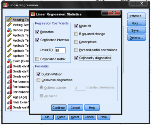
To answer our simple research question we just need to add the Math Test Score as the dependent variable and the Writing Test Score as the independent variable. The menu Statistic allows us to include additional information that we need to assess the validity of our linear regression analysis. To assess autocorrelation (especially if we have time series data) we add the Durbin-Watson Test, and to check for multicollinearity we add the Collinearity diagnostics.
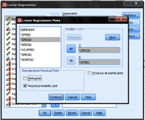
Lastly, we click on the menu Plots… to add the standardized residual plots to the output. The standardized residual plots chart ZPRED on the x-axis and ZRESID on the y-axis. This standardized plot allows us to check for heteroscedasticity.
We leave all the options in the menus Save… and Options… as they are and are now ready to run the test.

If you’re like others, you’ve invested a lot of time and money developing your dissertation or project research. Finish strong by learning how our dissertation specialists support your efforts to cross the finish line.
