Conduct and Interpret a One-Sample T-Test

What is the One-Sample T-Test?

The one-sample t-test is a member of the t-test family.  All the tests in the t-test family compare differences in mean scores of continuous-level (interval or ratio), normally distributed data.  Unlike the independent or dependent-sample t-tests, the one-sample t-test works with only one mean score.  The one-sample t-test compares a sample mean to a predetermined value to see if it’s significantly greater or less.

The independent sample t-test compares the mean of one distinct group to the mean of another group.  An example research question for an independent sample t-test is “Do boys and girls differ in their SAT scores? A dependent sample t-test compares two matched scores or measurements (e.g., before vs. after).  An example research question for a dependent sample t-test would be, “Do pupils’ grades improve after they receive tutoring?”

The one-sample t-test compares the mean score of an observed sample to a predetermined or hypothetical value. Typically, the hypothetical value is the population mean or some other theoretically derived value.

Some possible applications of the one-sample t-test include testing a sample against a predetermined or expected value, testing a sample against a certain benchmark, or testing the results of a replicated experiment against the original study.  For example, a researcher may want to determine if the average age of retiring in a certain population is 65.  The researcher would draw a representative sample of people entering retirement and ask at what age they retired.  You could conduct a one-sample t-test to compare the mean age obtained in the sample (e.g., 63) to the hypothetical test value of 65.  The t-test determines whether the difference we find in our sample is larger than we would expect to see by chance.

The Process in SPSS

In this example, we will conduct this to determine if the average age of a population of students is significantly greater or less than 9.5 years.

Before we actually conduct this process, our first step is to check the distribution for normality.  You can do this with a Q-Q Plot (located under Analyze > Descriptive Statistics in SPSS). Then we simply add the variable we want to test (age) to the box and confirm that the test distribution is set to Normal.  This will create the diagram you see below.  The output shows that small values and large values somewhat deviate from normality. We can run a Kolmogorov-Smirnov (K-S) test to check the null hypothesis that the variable distributed is normal. It helps to find that the K-S test is not significant, so we cannot reject the null hypothesis and can assume that age distributed is normal.

Let’s move on to it, which can be found in Analyze > Compare Means > One-Sample T Test…

The dialog box is fairly simple.  We add the test variable age to the list of Test Variables and then enter the Test Value.  In our case, the hypothetical test value is 9.5.  The dialog Options… gives us the setting for how to manage missing values and also the opportunity to specify the width of the confidence interval used for testing.

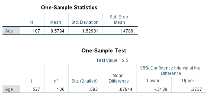
After setting all the appropriate options, click OK to run the analysis.  The figure below shows the output.  The following section shows descriptive statistics, including the mean being compared to the test value.  Also, it shows the results of the t-test.  In this case, the null hypothesis’ mean is equal to 9.5.  For the purpose of this example, we will set our significance (alpha) level to .05.  The Sig. column displays the p-value for the test.  The results show that the p-value (.592) is greater than .05.  This suggests that the null hypothesis cannot be rejected, and the age of the sample is not significantly different from 9.5.