Ordinal Association
Ordinal variables are variables that are categorized in an ordered format, so that the different categories can be ranked from smallest to largest or from less to more on a particular characteristic. Examples of ordinal variables include educational degree earned (e.g., ranging from no high school degree to advanced degree) or employment status (unemployed, employed part-time, employed full-time). Numeric variables that are presented in categories or ranges are also considered ordinal as it is not possible to perform mathematical functions on the grouped numbers. Examples of this type of ordinal variable include age ranges (<18, 19-34, >35) or income presented in ranges (<$20k, $20k-50k, >$50k). The examination of statistical relationships between ordinal variables most commonly uses crosstabulation (also known as contingency or bivariate tables). Chi Square tests-of-independence are widely used to assess relationships between two independent nominal variables.
Questions answered:
Does a relationship exist between income level and highest degree earned?
Is there an association between BMI scales and height categories?

Discover How We Assist to Edit Your Dissertation Chapters
Aligning theoretical framework, gathering articles, synthesizing gaps, articulating a clear methodology and data plan, and writing about the theoretical and practical implications of your research are part of our comprehensive dissertation editing services.
- Bring dissertation editing expertise to chapters 1-5 in timely manner.
- Track all changes, then work with you to bring about scholarly writing.
- Ongoing support to address committee feedback, reducing revisions.
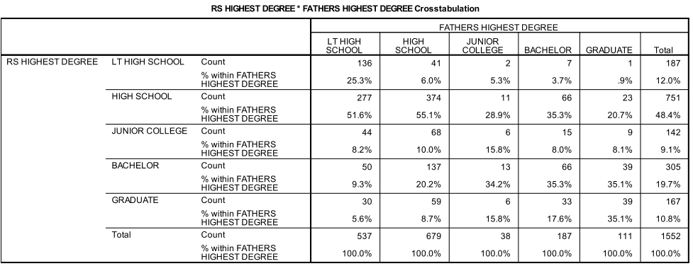
Unlike with nominal associations, crosstabulations between two ordinal variables show patterns of association and can also reveal the direction of the relationship between the variables. The direction of the relationship refers to a situation in which cases with high values on the independent variable are also likely to have high values on the dependent variable (a positive relationship) or low values on the dependent variable (a negative relationship). Essentially, if a high count in one category is related to a high or low count in another category of another variable. This is most easily observed by circling the highest count (usually given as a percentage) in each row and looking for the pattern of circles. In the following example, there is clear a line from the upper left portion of the table to the lower right, indicating a positive relationship. Note that direction can ONLY be determined when both variables are measured at the ordinal level, as there is no ranking of nominal variables.
SPSS provides a number of common measures of association for ordinal variables, some of which are directional (meaning the value of the measure depends on which variable is treated as independent) and some that are symmetric (without direction). These measures of association take advantage of the ranked nature of ordinal variables by observing pairs of observations in the crosstabulation and counting the number of untied concordant and discordant pairs. A concordant pair is one in which one observation has a higher rank on both variables than the other observation in that pair, while a discordant pair refers to a situation in which one observation ranks higher than the other observation on one variable but not on the other. Because these measures take into consideration the direction of the relationship, they can range from -1.0 to +1.0, with a value of 0 indicating no relationship.
As seen below, Somer’s d is primarily an asymmetric measure of association, meaning that whichever variable is treated as the dependent variables matters (though it can also be conceptualized as symmetric). Somer’s d is a Proportional Reduction in Error (PRE) measure so it is interpreted as the improvement in predicting the dependent variable that can be attributed to knowing a case’s value on the independent variable. A value of .346 for the crosstabulation above (treating the respondent’s education as dependent) indicates that we improve our guess of respondent education by 34.6% by knowing father’s education.
SPSS provides three common symmetric measures of association, with gamma being the most widely used. The value of gamma tends to be large due to how it is calculated, so tau-b (for square tables) or tau-c (for non-square tables – like a 2 x 3 table) are often preferred even though they are not PRE measures. Because the crosstabulation above is a square (5 x 5), we would report the tau-b of .34.. Because gamma is a PRE measure we can again say that knowing father’s education improves our prediction of respondent’s education by 48.4%.
Assumptions:
Adequate sample size for each of the categories being analyzed.
Variables must be ordinal.
If a zero is present in the crosstabulation, no association can be assessed.
Related analyses:


