The Multiple Linear Regression Analysis in SPSS
This example is based on the FBI’s 2006 crime statistics. We focus on how state size, property crime rates, and the number of murders in the city are related. It is our hypothesis that less violent crimes open the door to violent crimes. We hypothesize that an effect remains even after accounting for city size by comparing crime rates per 100,000 inhabitants.
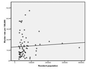
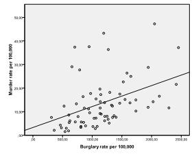
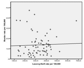
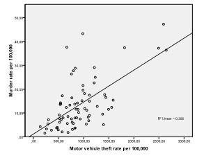
First, we need to check for a linear relationship between the independent and dependent variables in our regression model. To do this, we can check scatter plots. The scatter plots show strong linear relationships between murder, burglary, and theft rates, and weak ones between population and larceny.
Need help conducting your Multiple Linear Regression? Leverage our 30+ years of experience and low-cost same-day service to make progress on your results today!
Schedule now using the calendar below.
Secondly, we need to check for multivariate normality. We can do this by checking normal Q-Q plots of each variable. In our example, we find that multivariate normality might not be present in the population data (which is not surprising since we truncated variability by selecting the 70 biggest cities).
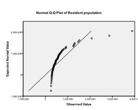
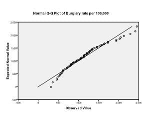
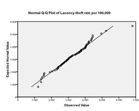
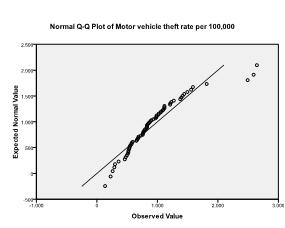
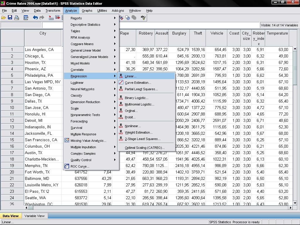
We will ignore this violation of the assumption for now, and conduct the multiple linear regression analysis. You can find multiple linear regression in SPSS under Analyze > Regression > Linear.
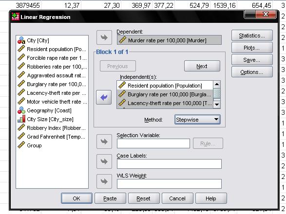
In our example, we enter “murder rate” as the dependent variable and population, burglary, larceny, and vehicle theft as independent variables. In this case, we will select stepwise as the method. The default method for the multiple linear regression analysis is ‘Enter’. That means that all variables are forced to be in the model. Since overfitting is a concern, we only want variables in the model that explain a significant amount of additional variance.
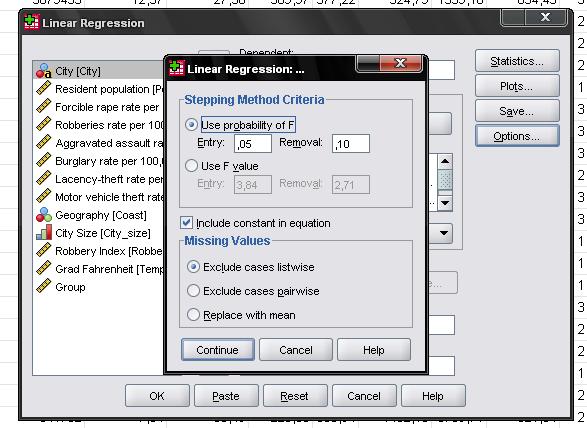
In the field “Options…” we can set the stepwise criteria. We include variables that increase the F-statistic by at least 0.05 and exclude those with less than 0.1.
The “Statistics…” menu allows us to include additional statistics that we need to assess the validity of our linear regression analysis.
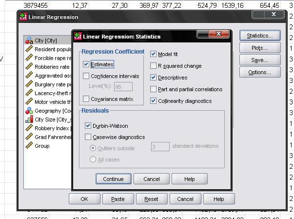
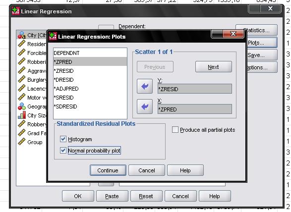
It is advisable to include the collinearity diagnostics and the Durbin-Watson test for auto-correlation. To test the assumption of homoscedasticity and normality of residuals we will also include a special plot from the “Plots…” menu.
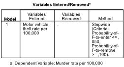
The first table in the results output tells us the variables in our analysis. Turns out that only motor vehicle theft is useful to predict the murder rate.
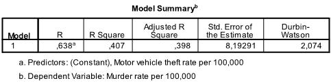
The next table shows the multiple linear regression model summary and overall fit statistics. We find that the adjusted R² of our model is .398 with the R² = .407. This means that the linear regression explains 40.7% of the variance in the data. The Durbin-Watson d = 2.074, which is between the two critical values of 1.5 < d < 2.5. Therefore, we can assume that there is no first order linear auto-correlation in our multiple linear regression data.
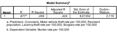
If we would have forced all variables (Method: Enter) into the linear regression model, we would have seen a slightly higher R² and adjusted R² (.458 and .424 respectively).
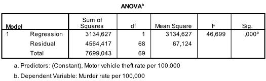
The next output table is the F-test. The linear regression’s F-test has the null hypothesis that the model explains zero variance in the dependent variable (in other words R² = 0). The F-test is highly significant, thus we can assume that the model explains a significant amount of the variance in murder rate.
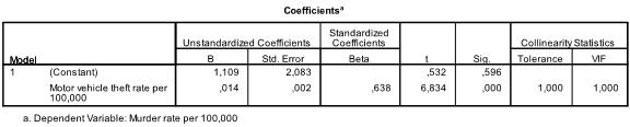
The next table shows the multiple linear regression estimates including the intercept and the significance levels.
In our stepwise multiple linear regression analysis, we find a non-significant intercept but highly significant vehicle theft coefficient, which we can interpret as: for every 1-unit increase in vehicle thefts per 100,000 inhabitants, we will see .014 additional murders per 100,000.
If we force all variables into the multiple linear regression, we find that only burglary and motor vehicle theft are significant predictors. We can also see that motor vehicle theft has a higher impact than burglary by comparing the standardized coefficients (beta = .507 versus beta = .333).
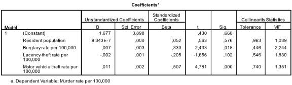
The information in the table above also allows us to check for multicollinearity in our multiple linear regression model. Tolerance should be > 0.1 (or VIF < 10) for all variables, which they are.
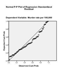
Lastly, we can check for normality of residuals with a normal P-P plot. The plot shows that the points generally follow the normal (diagonal) line with no strong deviations. This indicates that the residuals are normally distributed.
Take the Course: Linear Regression