Testing Assumptions of Linear Regression in SPSS
Starting on the journey of regression analysis in SPSS after collecting your data is a pivotal moment in any research project. Once you have meticulously prepared your dataset, as outlined in our guide on data cleaning and management in SPSS, you are now ready to dive into the regression analysis. Furthermore, this step not only allows you to explore the relationships between variables but also sets the stage for uncovering meaningful insights. In addition, it helps you test hypotheses and predict outcomes based on your dataset.
As a result, you can move from raw data to actionable conclusions, adding depth to your research. Moreover, understanding the key processes involved will enable you to confidently interpret the results and make informed decisions moving forward. However, diving directly into interpreting the regression results without a proper check on the underlying assumptions can lead to misleading conclusions. Let’s demystify the essential assumptions of normality, linearity, homoscedasticity, and the absence of multicollinearity, guiding you through each step with clarity.
Normality of Residuals:
The foundation of valid regression analysis lies in the normal distribution of residuals—the differences between the observed and predicted values of the dependent variable. To assess this, a normal Predicted Probability (P-P) plot serves as a valuable diagnostic tool. In particular, when the residuals follow a normal distribution, they will align closely with the plot’s diagonal line, indicating that the assumptions of the regression model are met. Additionally, any significant deviations from this line may signal potential issues with the model, such as non-normality or outliers. Therefore, this diagnostic check is crucial for ensuring the accuracy and reliability of your regression analysis. Moreover, if the P-P plot reveals irregularities, it provides a starting point for further model refinement or transformations of the data. We’ll illustrate how to interpret this plot effectively later on.

Homoscedasticity:
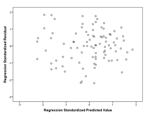
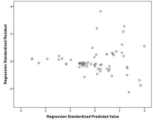
This assumption concerns the distribution of residuals. To ensure your data is homoscedastic, the residuals should spread evenly across the range of predicted values, resembling a “shotgun blast” of points. This uniform distribution ensures that the variance of errors is constant. Heteroscedasticity, the opposite condition, manifests as a patterned spread of residuals (e.g., cone or fan-shaped), indicating variance inconsistency. We will guide you on how to visually assess homoscedasticity through a scatterplot of predicted values against residuals.
Linearity:
The assumption of linearity posits a direct, straight-line relationship between predictor and outcome variables. If the residuals are normally distributed and exhibit homoscedasticity, linearity typically holds, simplifying the analysis process. Multicollinearity refers to when your predictor variables are highly correlated with each other. This is an issue. This hinders your regression model from linking variance to the correct predictor, leading to muddled results and incorrect inferences. Keep in mind that this assumption is only relevant for a multiple linear regression, which has multiple predictor variables. If you are performing a simple linear regression (one predictor), you can skip this assumption.
Absence of Multicollinearity:
In multiple linear regression, where several predictor variables are involved, multicollinearity can obscure the distinct impact of each predictor. This phenomenon occurs when predictors highly correlate with one another, complicating the attribution of variance in the outcome variable. Multicollinearity assessment can be approached through two methods:
- Correlation Coefficients: By constructing a correlation matrix among predictors, coefficients nearing or exceeding .80 indicate strong correlations, suggesting multicollinearity.
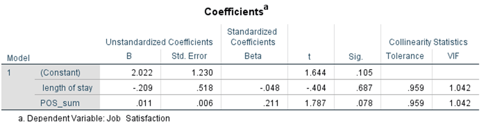
- Variance Inflation Factor (VIF): VIF values offer a quantitative measure of multicollinearity, with values below 5.00 indicating minimal concern, and those exceeding 10.00 signaling significant multicollinearity.
To fully check the assumptions of the regression using a normal P-P plot, a scatterplot of the residuals, and VIF values, bring up your data in SPSS and select Analyze –> Regression –> Linear. Set up your regression as if you were going to run it by putting your outcome (dependent) variable and predictor (independent) variables in the appropriate boxes.
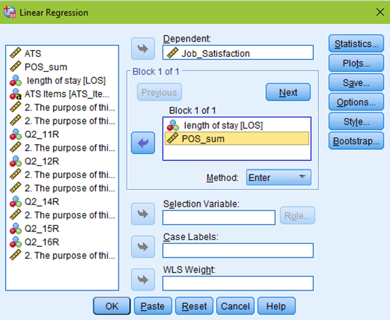
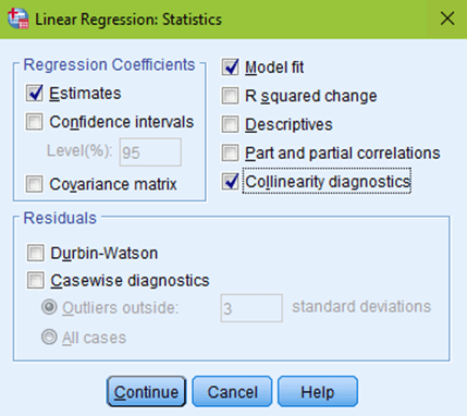
But don’t click OK yet! Click the Statistics button at the top right of your window. Estimates and model fit should automatically be checked. Now, click on collinearity diagnostics and hit continue.
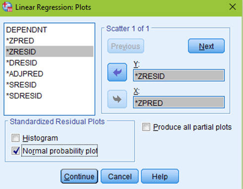
The next box to click on would be Plots. You want to put your predicted values (*ZPRED) in the X box. And your residual values (*ZRESID) in the Y box. Make sure to check the normal probability plot, then click continue.
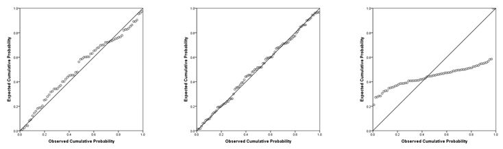
Now you are ready to hit OK! You will get your normal regression output, but you will see a few new tables and columns, as well as two new figures. First, you will want to scroll all the way down to the normal P-P plot. You will see a diagonal line and a bunch of little circles. Ideally, your plot will look like the two leftmost figures below. If your data is not normal, the little circles will not follow the normality line, such as in the figure to the right. Sometimes, there is a little bit of deviation, such as the figure all the way to the left. That is still ok; you can assume normality as long as there are no drastic deviations.
Evaluation of Homoscedasticity
The next assumption to check is homoscedasticity. The scatterplot of the residuals will appear right below the normal P-P plot in your output. Ideally, you should see a plot that, in this case, looks similar to the one below. The data looks like you shot it out of a shotgun—it does not have an obvious pattern, there are points equally distributed above and below zero on the X axis, and to the left and right of zero on the Y axis.
If your data is not homoscedastic, it might look something like the plot below. The plot shows a tight distribution on the left and a wide distribution on the right. If you were to draw a line around your data, it would look like a cone.
Evaluation of multicollinearity
Finally, you want to check absence of multicollinearity using VIF values. Scroll up to your Coefficients table. All the way at the right end of the table, you will find your VIF values. Each value falls below 10, confirming that it met the assumptions.
Report your assumption checking results in the results chapter, following school guidelines and committee preferences for detail. Err on the side of caution by including APA-formatted figures and VIF values in your results chapter. After testing these assumptions, you will be ready to interpret your regression!
Conduct and Interpret Your Analysis Quickly with Intellectus Statistics
Intellectus Statistics allows you to conduct and interpret your analysis in minutes. The system pre-loads assumptions and provides output in APA style, complete with tables and figures. Create a free account and start analyzing your data now!

If you’re like others, you’ve invested a lot of time and money developing your dissertation or project research. Finish strong by learning how our dissertation specialists support your efforts to cross the finish line.